This is the third post of the Recommendation Systems series. Here, we will discuss the Collaborative Filtering approach in recommenders, which is currently the industry standard in large commercial e-commerce websites and corporations.

Collaborative Filtering

Collaborative Filtering is considered the most prominent approach to generate recommendations in our days. The fact that it is used by large, commercial e-commerce sites and corporations is a reliable indication of its worth. Additionally, it is a well-understood technique with various algorithms and variations that enable it to solve many different types of problems.

The logic behind this technique is really simple. It uses the “wisdom of the crowd” to recommend items to users. In other words it uses data that shows the users’ preferences over some items, provided either explicitly or implicitly by the users, in order to recommend items that some users liked to users with similar tastes. This approach is built over the assumption that customers who had similar tastes in the past, will have similar tastes in the future.

Bellow, we will describe the 3 basic approaches of Collaborative Filtering, with examples for the most popular variations. What is common for all the approaches though, is that they expect a matrix of user-item ratings or interactions as an input and produce as output a numerical prediction indicating to what degree the current user will like or dislike a certain item.

Neighbourhood-based CF

The first approach that we will describe is the neighbourhood-based CF, because it has the most straight forward and easy to follow logic. There are two basic variations of algorithms used in this approach: the “User-based nearest neighbour CF” and the “Item- based nearest neighbour CF”.

**User-based nearest neighbour CF**

The basic technique for this category is based on the following logic. Given an “active user” and an item not yet seen by this user:

1. Findasetofusers(peersornearestneighbour)wholikethesameitemsasouruserinthe past and who have rated the given item.
   
2. Use, e.g. the average of their ratings to predict, if the given user will like the given item.
   
3. Do this for all the items that the given user has not seen yet and recommend the best- rated of them.
   

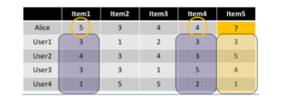
Let’s examine the algorithm described above with a simple example. If for example we have 4 users that have rated each one of a list of 5 items, and a fifth user comes (Alice) that has rated the 4 out of the 5 items and we want to predict if she is going to like the fifth item or not.

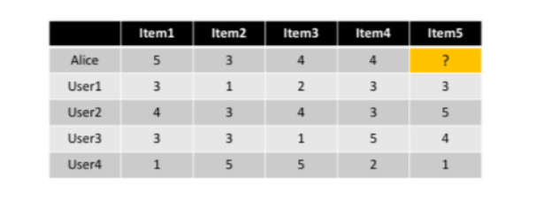
Seeing this table there are a few questions that come out, like:

• How de we measure similarity?
• How many neighbours should we consider?
• How do we generate a prediction from the neighbours’ ratings?

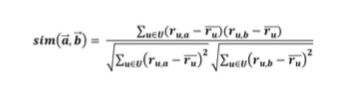
A popular similarity measure in user-based Collaborative Filtering is the Pearson Correlation which is computed according to the following formula:

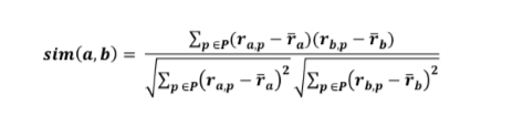
where a, b are the users, ra,p is the rating of user a for item p and P is the set of items, rated both by users a and b. The result is the similarity value which is between -1 and 1.

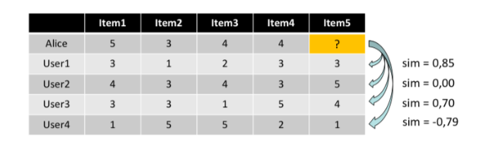
So, for the above example using the Pearson Correlation we can compute the similarity values between each user and Alice:

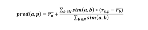
Now in order to produce the predictions, a common prediction function calculates, whether the neighbours’ ratings for the unseen item are higher or lower than their average. Then, it combines the rating differences using the similarity as a weight and finally, it adds or subtracts the neighbours’ bias from the active user’s average and use this as a prediction.

This is a general approach and of course some modifications or improvements may give us even better solutions. A first issue is that not all the items do they have the same value. It should be more important for the similarity between two users liking the same controversial item, than liking an item that is liked by many users. A possible solutions to this problem would be to give more weight to items that have a higher variance.

Another issue would be in selecting two users as similar when each of them have liked only a very small number of items and they agree on all of them. In order to deal with this, we could linearly reduce the weight when the number of the co-rated items are small.

Finally, another improvement could be achieved by using a similarity threshold or a fixed number of neighbours. In our first approach, we were taking each rating under consideration just with a weight that was computed from the users’ similarity. Making this change we would make our predictions to only look to the most similar neighbours instead of all of them.

With all these improvements we may be able to make really accurate predictions for the user preferences. But, still there is another issue we haven’t discussed, yet. What happens in large e-commerce websites that have millions of items and tens of millions of customers at the same time that new users are constantly arriving in the platform?

The kind of solutions we described above is called “Memory based”, because the rating matrix is directly used to find neighbours and/or to make predictions. Such algorithms do not scale good enough for most real-world applications. Thus, we need another approach which will enable us to use it in really big and scalable applications. There is another approach in neighbourhood based collaborative filtering and it is called “Model based”.

Model-based approach is based on an offline pre-processing or “model-learning” phase. Then at the run time, the algorithm only uses the produced model to make predictions. At the same time, periodically, models are updated and re-trained with all the new arriving data. There is a large variety of such techniques but we are going to concentrate to one of them, the “Item-based Collaborative Filtering”.

**Item-based CF**

The basic idea behind the Item-based CF is that it uses the similarities between items to make predictions, on the contrary to the User-based CF which uses similarities between users. The first thing that is making this approach better is that the most of the times the set of items is considered relatively small and stable while the set of users changes dynamically. and is by far larger than the set of items.

As we did with the User-based CF, we will start with an example to understand how this method works. Again we have 4 users, plus Alice and 5 items from which Alice had only tried and rated the 4 of them. Our goal is to predict the rating that Alice would give to the 5th item.

The algorithm is simple in this method, as well. We first need to look for items that are similar to item 5 and then take Alice’s ratings for these items to predict the rating for item 5. To compute the similarity between items we are going to use another technique this time, the cosine similarity measure. Cosine similarity produces better results in item-to-item filtering because ratings are seen as vectors in a n-dimensional space. The basic formula to compute the similarity is with calculations based on the angle between two vectors:

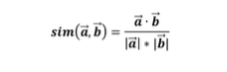
In order to have an even better solution, we can adjust the cosine similarity by taking the average user rating into account in order to transform the original ratings. In this case, the new function would be:

After we have calculated the similarities between items, the next goal is to define a prediction function. For example, a function for predictions could look like this:

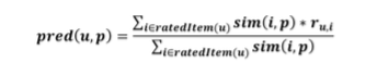
Of course, at this approach as well, the neighbourhood size is typically limited to a specific size. Thus, not all neighbours are taken into account for our prediction. Analysis has shown that in most real world situations, a neighbourhood of 20 to 50 neighbours seems reasonable.

Still, we haven’t analyse how the scalability problem is being solved in this method. The truth is that “Item-based CF” does not solve the scalability issue on its own. The keyword behind this solution is “pre-processing”.

Pre-processing for item-based filtering means that we have to first calculate all pair- wise item similarities in advance. Additionally, the neighbourhood used at run-time is typically rather small, because only the items that the user has rated are taken into account. So, it is obvious that pre-processing saves a lot of processing time in the run-time and if we also consider the fact that item similarities are supposed to be more stable than user similarities, we will understand why this method scales better.

As far as it concerns the memory requirements, this method needs n2 pair-wise similarities to be memorised, where n is the number of items. In practice, though, this number is significantly lower because items with no co-ratings are not taken into account. In addition some other reductions is possible to be done, like setting a minimum threshold for co-ratings.

Summing up, from the approaches we had analysed until now it seems that the best solution is the model-based technique of the collaborative filtering because it is more efficient during run-time and it scales better in big applications.

Rule-based CF

Rule-based algorithms are also used in recommenders systems in order to try to predict what items are possible that the user wants to select. Such algorithms are classified with the rest of the collaborative filtering methods since they use the “wisdom of the crowd”, or in other words past data gathered from all the users, in order to create some confident rules that describe users’ behaviour.

On the other hand, Rule-based algorithms does not create truly personalised recommendations. They are appropriate to understand that customers who buy pizzas is possible to order a bottle of Coca Cola as well, but this is not a recommendation made to a specific person.

The main technique used in this approach is the Association Rule Learning which is a rule-based machine learning method for discovering interesting relations between variables in large databases. It is intended to identify strong rules discovered in databases using some measures of interestingness. Based on the concept of strong rules, association rules were initially introduced for discovering regularities between products in large-scale transaction data recorded by systems like POS (Point-Of-Sales) in supermarkets.

For example, the rule {onions, potatoes} ⇒ {burger} found in the sales data of a supermarket would indicate that if a customer buys onions and potatoes together, they are likely to also buy hamburger meat. Such information can be used as the basis for decisions about marketing activities such as promotional pricing or product placements. Adapting this technique to recommendation systems, would help to analyse the electronic “basket” of each customer that will lead to a recommendation eg. proposing items to customer that are frequently ordered together with the items she have already selected.

Two of the well-known algorithms of this category are Apriori and FP-Growth, but they only do half the job, since they are algorithms for mining frequent item sets. Thus, another step needs to be done after their completion to generate rules from frequent item sets found in a database. Apriori uses a breadth-first search strategy to count the support of item sets and uses a candidate generation function which exploits the downward closure property of support.The second algorithm is the FP-Growth where the FP stands for Frequent Pattern. Given a dataset of transactions, the first step of FP-growth is to calculate item frequencies and identify frequent items. Different from Apriori-like algorithms designed for the same purpose, the second step of FP-growth uses a suffix tree (FP-tree) structure to encode transactions without generating candidate sets explicitly, which are usually expensive to generate. After the second step, the frequent item sets can be extracted from the FP-tree.

One of the most used frameworks when we talk about scalable applications is the Apache Spark. Spark implementation for association rules uses a parallel version of FP- growth called PFP which distributes the work of growing FP-trees based on the suffixes of transactions, and hence it is more scalable than a single-machine implementation.

Of course there are many other algorithms that belongs to this approach but there is no point in getting into more details since as we said in the beginning of this chapter rule based algorithms are not as “personalised” as we would want them to be. Still, it is a good alternative method that can of course be used in a hybrid variation of every other approach mentioned in this paper.