In this last post of the Recommendation Systems series, we will discuss the Matrix Factorization Collaborative Filtering approach in recommenders, which is probably the most used approach in the industry in our days. This method can be used with either explicit or implicit feedback from users, because as we have seen in both cases the user-item interactions are stored as a sparse matrix.

Matrix Factorization

Collaborative Filtering is considered the most prominent approach to generate recommendations in our days. The fact that it is used by large, commercial e-commerce sites and corporations is a reliable indication of its worth. Additionally, it is a well-understood technique with various algorithms and variations that enable it to solve many different types of problems.

The high-level idea behind matrix factorisation is quite simple. Having a user-item interaction matrix, we can decompose it into two lower rank matrices U and I. And we will decompose it in a way that the product of user-factors vector and item-factors vector could be transformed back to the number which represents user-item interaction in original interaction matrix.

At first we will start by analysing how the Matrix Factorisation work using explicit-type of feedback because this problem is the most researched and an easier concept to understand. But then, with some more details we are going to analyse the differences with when we work with implicit-type of feedback and we will present a similar approach to the one used for explicit feedback that covers the new parameters.

Working with Explicit feedback

At this point we need to refer to the Netflix Prize competition which was an open competition for the best collaborative filtering algorithm to predict user ratings for films, based on previous ratings without any other information about the users or the films. This competition was a huge motive for scientists to work on collaborative filtering algorithms and thus, it was responsible for the major breakthrough in this area.

Scientists, on this competition worked with explicit user feedback and one of the most popular solutions contained the decomposition shown bellow:

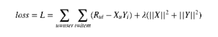
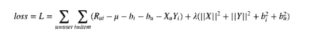
where R - observed ratings, X- user embeddings, Y- item embeddings and λ is regularisation parameter. A little bit more complex model could take general bias and biases for users and items under consideration:

Both of these models can be solved with different methods such as SGD and ALS. In the context of recommendation systems this decompositions is known as “SVD” but this is not accurate. In reality the famous “SVD” algorithm is the decomposition described above solved with the SGD method.

Although the largest part of the research made on Collaborative Filtering algorithms of Recommender Systems is concentrated on the explicit type of feedback, maybe thanks to Netflix Prize competition, we have to keep in mind that most real world applications on this field have to deal with implicit feedback. So the next question we need to answer is what would be an alternative approach to the one described above that can work for implicit feedback, as well?

Working with Implicit feedback

“Weighted alternating least squares” model which is described in Collaborative Filtering for Implicit Feedback Datasets paper has become the de-facto industry standard for matrix factorisation in implicit feedback settings. This can be proved by the fact that all the known Big-data frameworks like Spark and Flink have this method implemented and used by default in collaborative filtering problems that deal with implicit feedback.

The main idea is similar to “SVD” approach that was described above but have some differences on how we handle the numbers of the user-item interactions table. The first difference is that working with implicit feedback leaves us with no negative feedback. By observing the users behaviour, we can infer which items they probably like and thus chose to consume. However, it is hard to reliably infer which items a user did not like. For example, a user that did not watch a certain show might have done so because she dislikes the show or just because she did not know about the show or was not available to watch it.

A second difference is that the implicit feedback is inherently noisy. While we passively track the users behaviour, we can only guess their preferences and true motives. For example, we may view purchase behaviour for an individual, but this does not necessarily indicate a positive view of the product. The item may have been purchased as a gift, or perhaps the user was disappointed with the product after he received it.

Another difference is that the numerical value of explicit feedback indicates preference, whereas the numerical value of implicit feedback indicates confidence. Systems based on explicit feedback let the user express their level of preference, e.g. a star rating between 1 (“totally dislike”) and 5 (“really like”). On the other hand, numerical values of implicit feedback describe the frequency of actions, e.g., how much time the user watched a certain show, how frequently a user is buying a certain item, etc. A larger value is not indicating a higher preference. For example, the most loved show may be a movie that the user will watch only once, while there is a series that the user quite likes and thus is watching every week. However, the numerical value of the feedback is definitely useful, as it tells us about the confidence that we have in a certain observation. A one time event might be caused by various reasons that have nothing to do with user preferences. However, a recurring event is more likely to reflect the user opinion.

Having these differences in mind, in this case this is what we need to optimise:

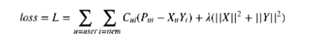
where X, Y are users and items embeddings.

In order to explain what are matrices P and C let’s first introduce matrix R which is the user-item interactions matrix. It is not presented in the equation above but it implicitly defines matrices P and C:

• P is indicator matrix where P[u, i] = 1 if user u interacted with item i and 0 otherwise.
• C is the most interesting part, the confidence matrix. It can be derived from R with a family of functions with signature C = 1 + f(R). Here, number 1 is a very important constraint cause it allows us to implement efficient optimisation algorithm which will be described below.

Authors of the model propose C=1+αR, where alpha is some hyper parameter. We can think that for the observed user-item interactions we are more confident that user will prefer this item over not observed item (which is very logical). For example, let α=40. In this case, Cui will be equal to 1 for non-observed user-item interactions and 40 ∗ rui for the observed interactions. As it is obvious, developers can design a wide range of functions to construct confidence from raw user-item interactions.

Having defined loss function, we have to now optimise parameters X and Y. As seen from the equation the problem is non-convex, which means that there is no efficient solver with convergence guarantees. SGD has been proved to be useful in such settings and can find a good local minimum but it also has some limitations: it is not easy to parallelise, implicit feedback datasets usually can be not very sparse, an additional hyper parameter - the learning rate - exists.

Alternatively, we can note that fixing X or Y makes problem convex. And we can leverage efficient techniques to solve the optimisation problem. So we can fix X, then compute approximation of Y then fix Y and compute approximation of X and so on. This method is called “Alternating Least Squares” and it is the most appropriate method for optimising the loss function we described above. And as we have already explained in the beginning of this chapter, this method is the standard method that is by default implemented my the major platforms out there that work with Big Data.

Conclusion

Recommender systems are systems that help users discover items they may like. They are used by companies because such systems can turn people who just browse the internet into buyers, can improve cross-sell by suggesting additional products for the customer to purchase and the most important they can help gaining customer’s loyalty which is an essential business strategy.

To succeed their goal, recommenders try to exploit every piece of information they have on the interactions between users and items. This information can be either explicitly provided by the customers who rate a set of given items or can be implicitly collected by monitoring every action a user makes. A general problem, that needs to be addressed is the cold start problem, which occurs when a new item is introduced in the store’s inventory or when a new customer is signed up and that is because of lacking history data for each new entity (user or item).

The are many methods that can use the information a company had collected about their items and their customers in order to provide some value through personalised recommendations. Knowledge-based algorithms requires perfectly knowing the each product’s features and each customer’s preference for each feature. Knowing all these details could deliver the most accurate recommendations. Content-based algorithms only require knowledge on how much a user prefer each item and on each product’s features. The rest of the work can be done by the algorithm which can understand the tastes of each customer and then provide an accurate set of recommendations.

However, there are some drawbacks in these methods. First of all, they have issues on scaling and thus, they cannot perform well in an online way. Additionally, in the general case companies cannot know each specific user’s tastes and analysing each and every feature of all the products can be very costly and make the system run too slowly.

A different approach is the Collaborative Filtering family of algorithms. Such methods use the past interactions between users and items to either come out with some general rules (Rule-based algorithms) on users’ behaviour or to provide some personalised recom- mendations by finding what items are preferred by users that have similar tastes or what items attract similar users (Neighbourhood-based algorithms).

Last, but not least, we have the Matrix Factorisation technique of Collaborative Filtering. This technique is the most scalable among the others and it can be used efficiently in an online way cause it produces a model that can be quickly accessed to provide real-time feedback. There are optimisations for both explicit-type of data (SVD algorithm) and implicit-type of data (ALS algorithm). In Netflix Prize competition, a competition that lead to major breakthrough in this “chapter” of Machine Learning, this family of algorithms proved to be the best way of handling such problems and that is the reason that they are the industry standard in our days.